Routemaster is a simple bus prediction model built in R & Azure designed to detect the presence of London Buses within TFL’s JamCams API feed. It utilises serverless Azure custom handler functions to run R code on a schedule, an Azure custom vision object detection model and R Shiny for the frontend (this website).
In short, the creation of Routemaster can be broken down into four core steps: scheduling the capture and storage of images from TFL’s API; training an object detection model; scheduling the submission of images for prediction and storing results; using the prediction results in a frontend application.
The following is a walkthrough on why and how I made Routemaster, as well as final thoughts on issues faced during its’ development and things I’d like to do differently. Each of the core steps is described, although some aspects like creating an Azure account, a resource group or storage account is skipped as Microsoft has numerous tutorials on these aspects.
The repository with all code used can be found on my Github account which is linked at the bottom of this page.
Why did I make Routemaster
Recently I started Microsoft’s learning pathway towards the Azure AI Engineer Associate certificate, and within this I learnt more about Azure’s computer vision solutions as well as discovering a demo of its’ capabilities. Having never used Azure’s custom functions or Azure’s custom vision models, I wanted to create a small end-to-end project following a similar approach using my preferred language – R.
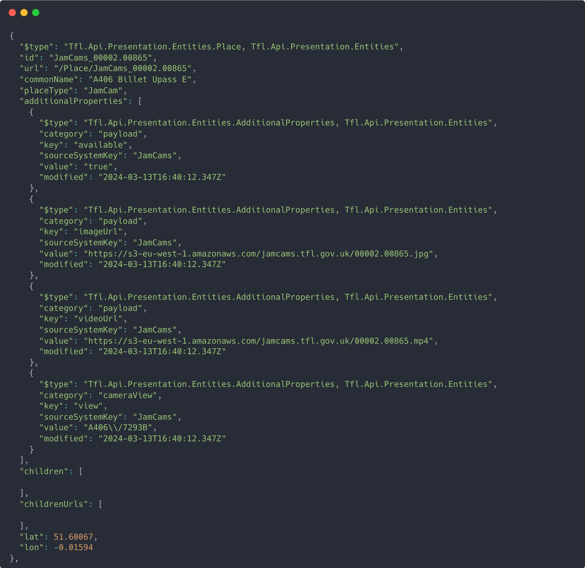
My only other self-imposed requirement was that I wanted to use real world data that was regularly updated or on a feed. Having previously used TFL’s APIs whilst at Parliament, I knew that they had free public endpoints which included their JamCam API. This API essentially exposes 10-second camera feeds and stills from 900+ traffic monitoring cameras from all over London with each camera updating roughly every five minute. A sample of the API is shown below.

From here I honed in on the idea of detecting buses within the images captured from the API largely as I thought it would be easier to build the object detection model on a form of traffic which is so identifiable – especially important with the small pixel count and low quality images from the camera feeds.
The result is a project which enabled me to develop some new skills, apply existing knowledge in different ways, and gain additional practical experience in implementing teachings from the Azure AI Engineer pathway.
Capturing JamCam images
To capture and store images from the JamCam API we need to write a relatively simple R script which goes through the URLs for the cameras we are interested in. I chose just three in this project for simplicity and cost reasons but in principle this can be extended to the full range. The script should copy the images to a blob storage container so that we have a record of which images were sent to the detection model as TFL does not keep past images/video feeds viewable – they are essentially overwritten each time TFL updates the feed.
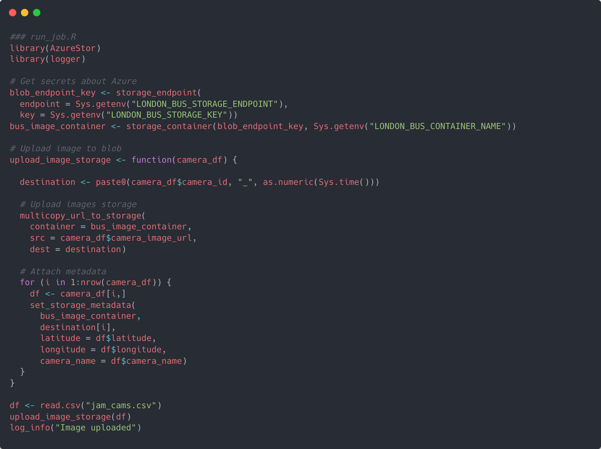
First of all, we need to create an Azure account, subscription, storage account and blob container where we can put the images. Next up is to create a new R project/directory with renv enabled to manage dependencies and to write a simple script like the one below which will grab and store our images using a package called AzureStor. I called my project image_timer_upload – the timer being a reference to a function we will make in a bit – and the script run_job.R.

Let’s talk through the script. It first creates a connection to the storage account and blob container which will store the TFL images by using the storage_endpoint and storage_container functions. For the endpoint argument you need the endpoint for your blob container which looks something like this yourstorageaccount.blob.core.windows.net as well as the access key and container name. I stored these values in a .Renviron file.
The rest of the script is centred on a function called upload_image_storage. This takes as a single argument the dataframe with details on the TFL cameras you’re using (camera IDs, camera names, longitudes, latitudes and image URLs). Within the function, a unique destination name is generated by a combination of the camera ID and current system time, followed by the actual upload to your blob container with the multicopy_url_to_storage function. Once uploaded, the function creates metadata for the blobs with the set_storage_metadata function.
If you were to run this script the end result should be a number of blobs in your container which would be the images from the API.
Scheduling the upload
To automate the running of this script we are going to take advantage of Azure Functions which, like AWS Lambda, is an event-driven serverless offering which allows us to run code without provisioning or managing servers. This is easier for languages like Python, C# or Javascript as Azure offers support for these by default but for other languages, including R, we need to create a custom handler which will execute our function.
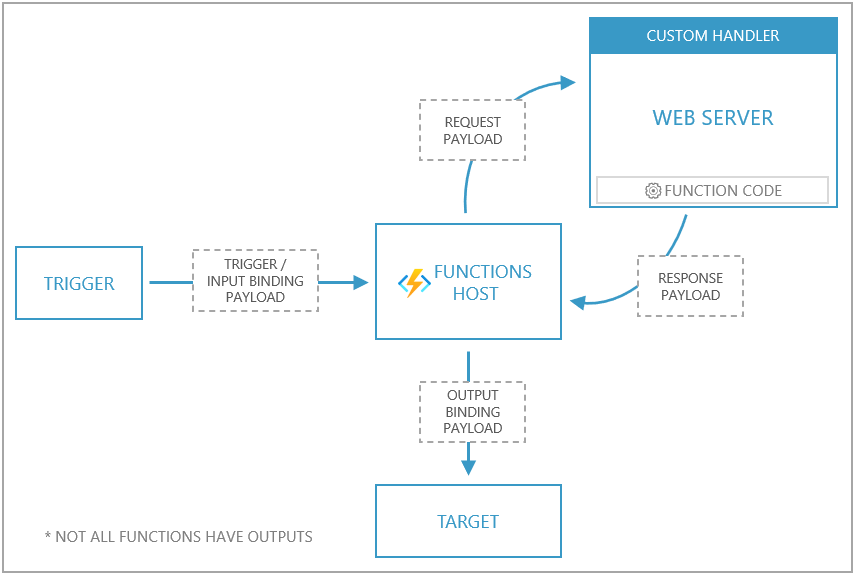
Custom handlers are lightweight web servers in your chosen language that receive triggers from the functions host, and then acting on these event triggers runs the code you want executed. The functions host and the custom handler are actually ran from inside the same single Docker container, and it's this which we will eventually use in Azure. For the purposes of this project I used the timer trigger to schedule when to run our script. Microsoft provides the following diagram to explain how custom handlers work. For more information on custom handlers see Microsoft’s documentation.

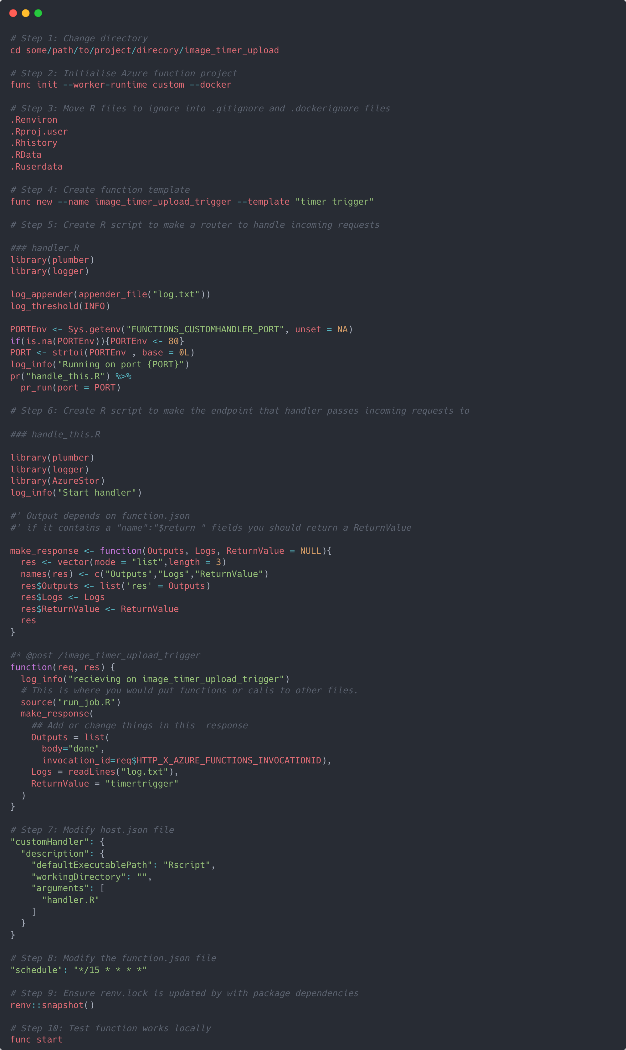
To create this custom handler, we first need to make sure we have Azure functions core tools, Azure CLI, and Docker installed on our machine. Once installed, go to the terminal and cd to the directory where our R project is located, then initialise a new Azure function project.
This will create some new files in the project directory: .gitignore, local.settings.json, vscode/extensions.json, a boiler plate Dockerfile and a .dockerignore. The next part is to copy the R files listed in to both the .dockerignore and .gitignore - this will make sure we aren’t sharing anything sensitive when we build and push our Docker image to a container registry.

Next up is step 4. This creates a new folder in the directory that holds a file called function.json which is the template with the settings of the actual trigger we’re using. I called mine image_timer_upload_trigger.
We now need to create two more R scripts. The first will act as the router which will handle incoming requests to the server directing them to a corresponding endpoint. The second will create an endpoint which will receive these incoming requests directed by the handler and effectively hits the endpoint making it run the R code we’re actually interested in.
Step 5 creates the router in a script called handler.R, and step 6 creates the endpoint in a script called handle_this.R. In the last couple of lines of handler.R you’ll see it’s ‘plumbing’ the incoming request through to handle_this.R which in turn is creating an endpoint in R with @post /image_timer_upload_trigger. When this endpoint is hit it’ll run the function associated with it, and it’s in here that we place the run_job.R script we made earlier. Essentially it’s saying whenever the /image_timer_upload_trigger endpoint is hit with a POST request please run our R script.
Now we need to tell our Azure function project how to run our custom handler. Go to the host.json file and change the defaultExecutablePath to be an Rscript, and the arugments to include the handler.R file – see step 7. This makes sure that the Azure function knows that it needs to execute an R script and which one to run.
In step 8 we change the function.json file to be the schedule we want it to be. The format of the schedule follows CRON syntax – a great tool to see what any given schedule will be with CRON is with crontab.guru. I set my schedule to be every 15 minutes, although it can be as frequent as you like.
Next, make sure you run renv:snapshot() to ensure that all the packages we’ve used in our R scripts (along with their dependencies) are recorded and saved in the renv.lock file.
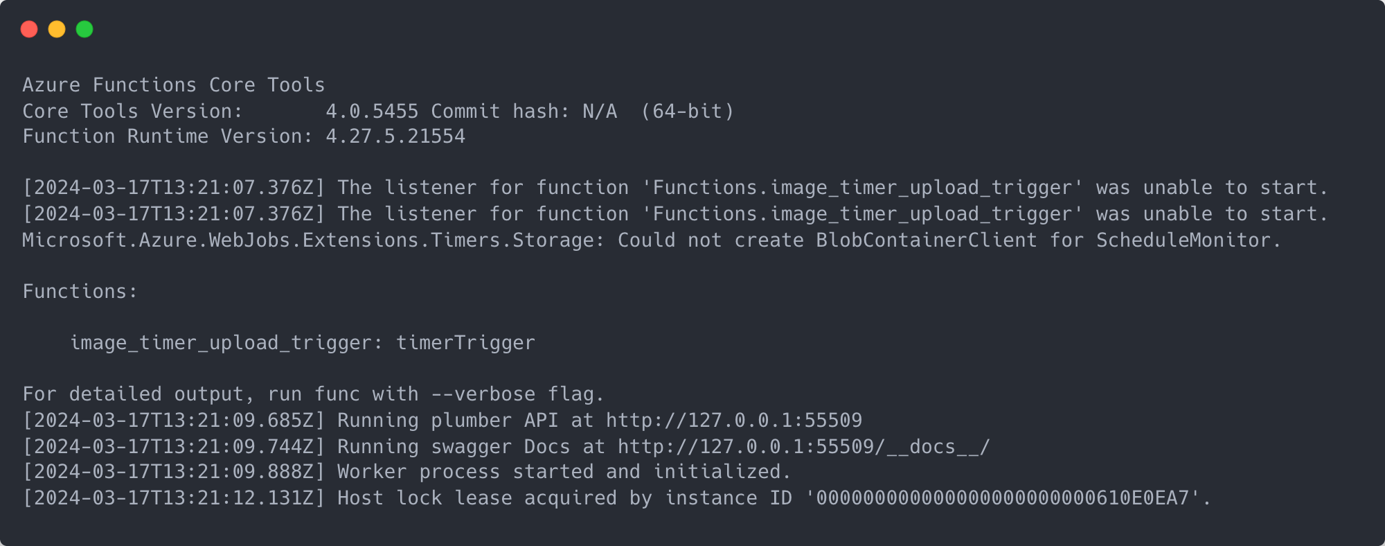
Now we can test the function works locally (step 10). In the terminal run func start. This will start running the Azure function locally, and eventually you should see some output like in the example below. Ignore the errors around the function being unable to start because it couldn’t connect to storage (we’ll sort this out later). You should eventually see that the timer trigger is running at an address which you can visit in your browser. If we go to the address for the Swagger docs, you’ll see the API endpoint we created in step 5. You can try the endpoint out by clicking ‘Try it out’ and then pressing ‘Execute’. This will then run all the code within our run_job.R file and if you were to look in the blob container we’re copying TFL’s images to you should see new blobs created. Notice that by running this function locally and manually executing a POST request we are ignoring the CRON schedule adjusted in step 8.

Dockerfile
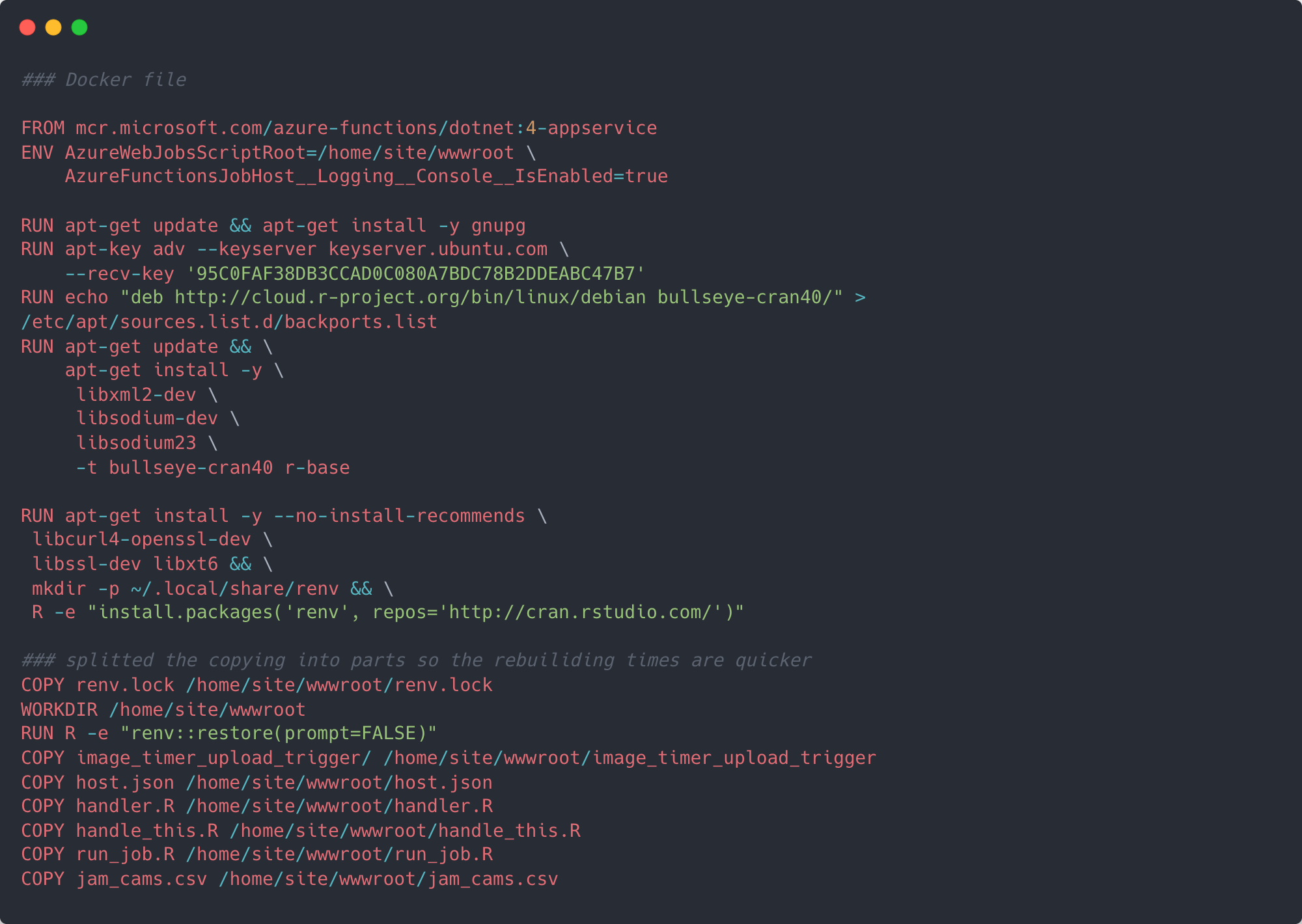
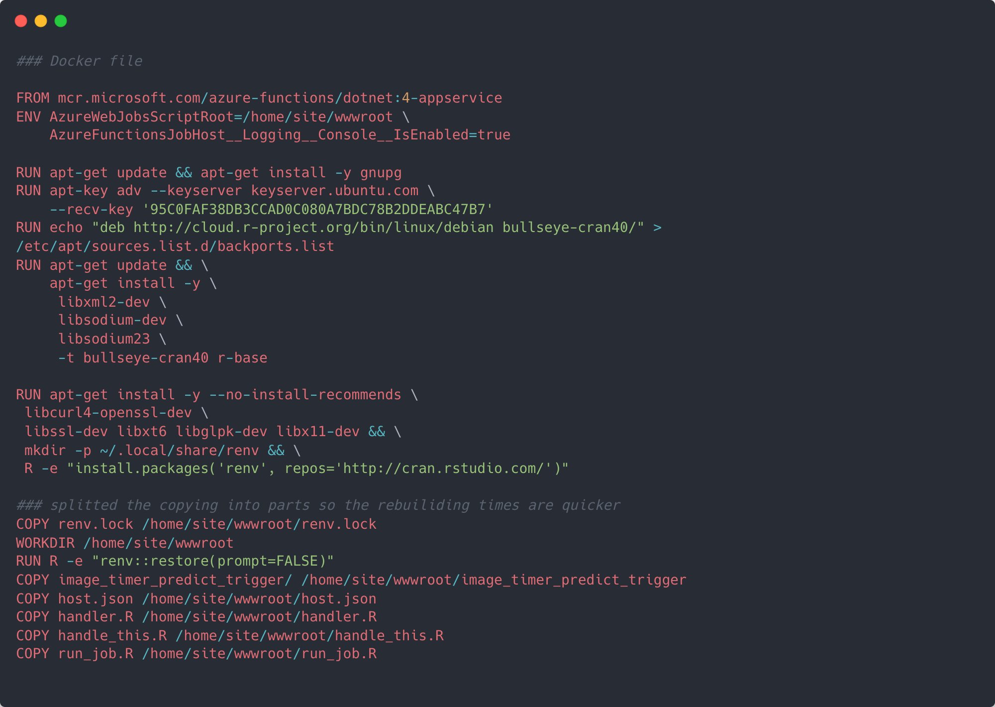
Now we’ve got the function running locally, the next step is to edit the Dockerfile created in step 2. To get Azure functions to run custom handlers everything needs to be inside a container. It’s this Dockerfile which helps us define what the eventual container should look like. Before we begin, make sure you have Docker installed and running and copy the following Docker code.

When we initialised the function project, Azure created a boiler plate Dockerfile with a base image required to run Azure functions in a container and interact with the rest of Azure’s framework. At time of writing all Version 4 Azure function docker images are based on Debian 11 (“Bullseye”).
Knowing this, we can make sure we install the correct version of R from the Debian repository, as well as any other required dependencies. Next, our Dockerfile will make sure it has renv installed so that it can install all the correct versions of the R packages we used. Finally, it copies the files from our directory into /home/site/wwwroot/ of the container.

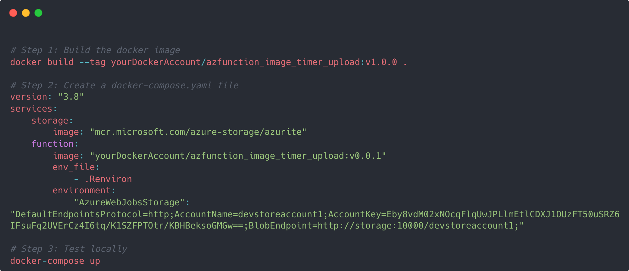
Now it’s time to build the docker image and test it. First, use Docker’s build function to create an image in your Docker account along with an appropriate name. I called mine azfunction_image_timer_upload. As we’ve used a timer trigger (which requires a storage account – hence the error when we tested locally last time), we need to make a dummy storage account that our function can connect to.
Create a text file called docker-compose.yaml in your directory and copy in the details from the example below. Under the hood this is effectively going to create two docker containers – one for our function, and one for the dummy storage account. After you’ve made the YAML file, run docker-compose up up in the terminal. Once the Docker containers are up and running go into the main Docker application and view the container in the container tab. In there you should see a short host address 8080:80 which if opened in your browser should be a stock page from Azure indicating that the function is running. Depending on the CRON schedule you made you should begin to see blobs being created in your chosen blob container.
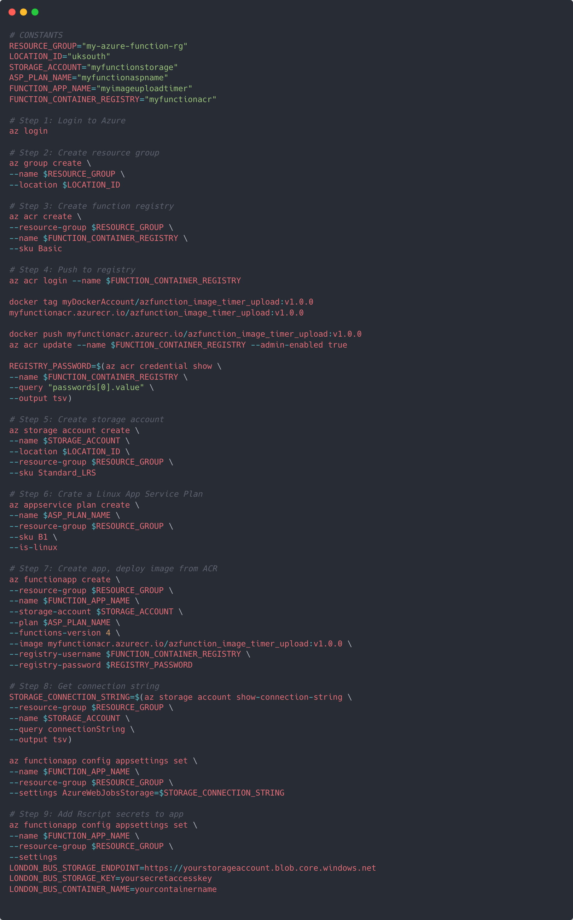
Next we will push everything to Azure by going through each step in the example shell script below. Within this script we are going to define some variables, create a new resource group to hold everything to do with the running of our Azure function, create a container registry to hold our Docker container, create the storage account that the timer trigger needs to run, create a new function app to run our container application, an app service plan for us to bill against, connect the storage account to the function app, and add our secrets to the environment.
Once everything is complete, you should be able to go to your Azure account and see all the new resources created as well as whether they are running. For specific details on the resources created refer to Microsoft documentation.

Training the model
Creating the model is simple - all we must do is sign in to Azure custom vision, create a new project and specifying that we would like to make a multi class object detection model. Once this is set up, we can add images to the project and begin a process of manually tagging buses. In this project I downloaded around 6,000 images from the JamCam API to my local machine and added them to the bus model project over the course of one weekend.
Once you’ve tagged a few hundred images we can take advantage of the Smart Labeler which is a model in its own right – this will go through and add tags to uploaded images itself which you can then accept or decline. Overall, 1,000 training images were tagged with buses and I had four training iterations. After each training iteration I added more photos for tagging and retrained. In the first iteration the model had an 88.6% mAP, and by the fourth iteration this had increased to 94.5%. In your model you may have different values. Whilst the model I made could certainly be improved, for the purposes of this project the actual performance of the model wasn’t my primary concern..
Once the model has been trained to a level you’re happy with, we can publish it get access to its’ endpoint and access key. These are what we’ll need to in order to submit new images for prediction.
Submitting images for prediction
We’ll be using another custom handler function with a timer trigger to submit images stored in our blob container for prediction and to store the results. The steps from earlier section are all relevant here and can be followed again changing references to the old function name with a new one – for instance I called this new function image_timer_predict. The main differences between this new scheduled function and the previous are within the main R script and the Dockerfile.
This is a much larger R script than before and does several more tasks – notably it submits images for prediction and retrieves the results, draws prediction bounding boxes on images and notes the probability score for each detection, and updates two small .csv files to count the total number of buses seen as well as the latest nine bounding box (what I called annotated) images.
The first part of the script connects to three new blob containers made in the main storage account as your original blob container. These hold the prediction results, the annotated images, and summary data. Next, the headers for the model endpoint are constructed, and the unique IDs/names for latest three blobs captured from TFL are retrieved. We also need to add in a token to allow the model to actually view the image that’s in our blob container. For this project I generated a read only SAS token for the blob container with a long expiry (I will explain reasoning for this later). By adding the token to the end of the URL for a given image in the blob container we can allow any other people or applications read access to the blob.
We then iterate over each image and send to the model in the body of the request, and store the returned predictions in a dataframe. Within this dataframe we are capturing the probability score for any detected object and the bounding box coordinates. I’m also filtering the returned predictions to only keep those that are equal or greater than 75%. Once all images have been submitted and predictions returned we upload the dataframe as a .csv to the relevant blob container using the storage_write_csv function.

Next, we download and update the prediction_summary_df.csv which contains a simple tally of the number of bus predictions the model has made. This is then reuploaded to the relevant blob container and the downloaded file is deleted.
To annotate the prediction bounding boxes we download the images which had just been submitted for prediction, iteratively load the image into R with the imager package, transform it so it can sit nicely in ggplot and add a bounding box for detected objects. Note that the bounding box coordinates returned from the model are actually percentage values based on the image size, and so we must multiply them against the width and height of an image to get the correct x, y coordinates. Once all bounding boxes are drawn on any image we save the plot as a new image and upload to the blob container.
We download and update a .csv file containing the paths (with SAS token) of the latest nine annotated images (annotate_summary_df) which we will use in our R Shiny application. For the Dockerfile, it’s almost exactly the same although two key libraries libglpk-dev and libx11-dev are needed to get imager working with Ubuntu.
Finally, we can re-run through the shell script from earlier although this time we ignore steps 2, 3, 5 and 6 as well as changing the FUNCTION_APP_NAME and adding in additional environment variables in step 9. Again, once everything is complete, you should be able to go to your Azure account and see the new function created as well as the predictions and annotated images being stored in the relevant blob containers.

Creating the Shiny App
For this project I've opted to use Shiny with a HTML template to showcase model outputs. Using Shiny this way allows us to generate more complete web pages (not solely a dashboard), but still allows us to include Shiny components. Posit's Shiny guides detail exactly how to use templates, although essentially all that needs to be done is to reference the template in the ui component of your app, and ensure that Shiny components by placing elements within two pairs of curly braces. An overview of how all these interact with each other for this site is shown below.

When the app is initiated several lines of code are ran before the creation the ui and server components. Let's look at these in turn. Firstly, connections to our blob containers in Azure are made in the same way we've done already using AzureStor. Specifically, they are just connecting to the blob containers that hold our summary data on the number of predictions made and the container holding the annotated images with predictions.
After these connections are made the ui and server components are created. The server component is more important for this project as it holds the code to read in the prediction_summary_df and annotate_summary_df files and gets the number of predictions made for each camera as well as the URLs of the annotated images to source. Both of these are held in a reactive object. Several observe functions are used to 'observe' when the prediction_summary_df and annotate_summary_df are updated and 'eagerly' sends new values rendered from the server to the client in the ui.
The ui component has less to do, as it's mostly just holding a reference to www/index.html (the template), as well as linking the rendered outputs generated in the server to a variable that the index.html will be looking for when it enounters the same name between curly braces.
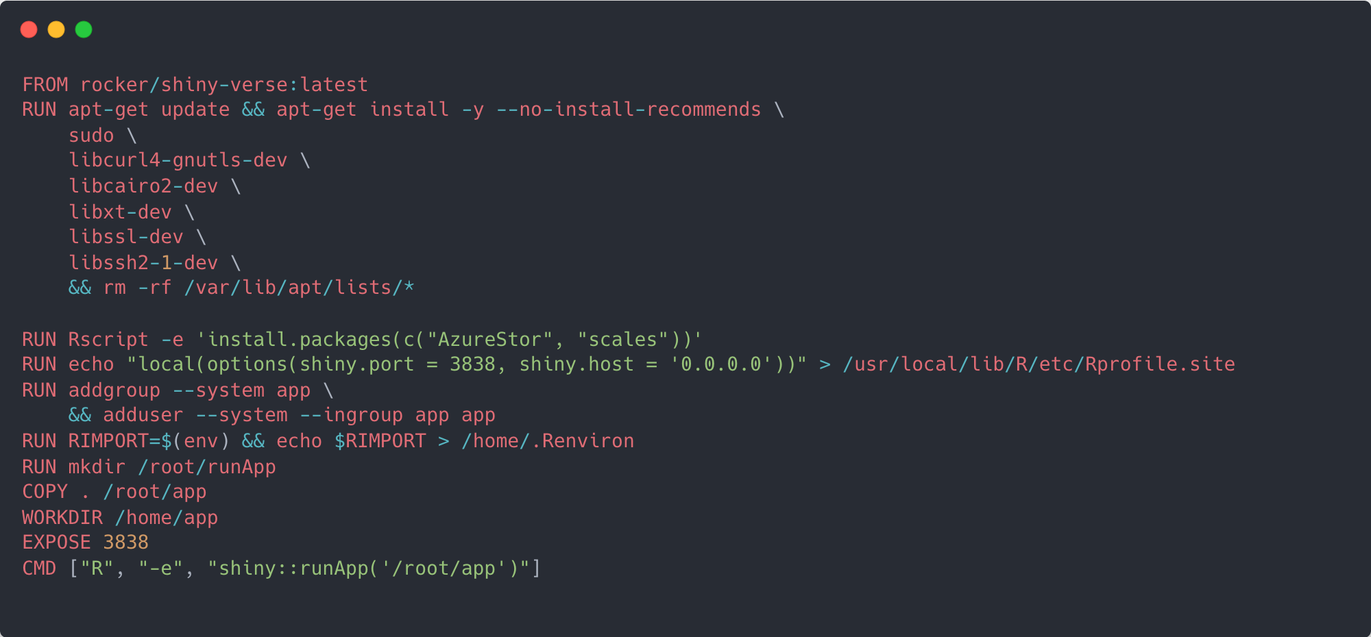
With all the components working with each other we can write a Dockerfile like in the example below, and then build, push and deploy the image/container to a new Azure container registry and a new app service plan. I decided to keep these seperate from the ACR and ASP created for the Azure functions as they, in my mind, are conceptually a different part of the pipeline. Once this is all done, you should be set and able to visit the deployed website!

Final thoughts
To recap, we've just gone through how this project and this site was made. We scheduled the storage of images from TFL's JamCam API with the use of Azure functions, made a custom object detection model with Azure Vision, automated prediction and result collection, and finally built a Shiny application as a frontend. All of this was done in R and Azure.
Throughout this process there were a few design choices that I feel need clarifying as I'm not totally happy with some compromises that I needed to make.
SAS token - the first is the use of a SAS token with a considerably long expiry. In order to submit the images stored in blob to the model's API endpoint we needed to attach a SAS token to the end of the image URL to give the model 'permission' to read it. The same is true for when we source the annotated images to be used within this site. In an ideal world, I would have generated a new SAS token with a very short expriry for each image submitted to the model, and for each annotated image sourced here. Whilst having a SAS token with a long expiry means I don't have to keep on generating a new one it carries an obvious security risk - if anyone was able to get hold that token they too would potentially be able to gain read access.
The AzureStor package documentation gives details on how to generate new tokens programmatically, however, the tokens generated were seemingly invalid. This is an issue that others seem to have had. I've submitted an issue on the AzureStor Github pages although without response as at 21 March 2024. If in the future I'm able to generate new SAS tokens I'll look to revisit this project and amend as appropriate.
SQL server - the second issue I'm not entirely happy with is the use of .csv files to store prediction results. I had explored creating a SQL server database to append new prediction results to, and whilst I could connect to the SQL server I created locally in R it became more difficult within the container produced as a result of the Azure function. From investigation I think it may be due to drivers not being found. Again, in an ideal world I would have preferred the use of SQL to store all prediction results.
Number of cameras - when I started this project I had hoped to be able to submit images from all TFL's JamCam cameras to a model for prediction every 5 minutes (in line with the update from TFL). However, the costs associated with doing this, at least based on my understanding and interpretation of Azure's pricing, would mean this project would very quickly get too expensive for an individual to maintain longterm. According to Azure's Custom Vision pricing it costs £1.57 per 1,000 prediction transactions. At the moment I'm submitting 3 camera images 4 times an hour 24 hours a day for a total of 8,928 prediction transactions per month which should cost around £14. Increasing just the frequency of model submission for the same 3 cameras to every 5 minutes (12 times an hour) would equate to a monthly cost of £42. This price would only get higher with additional cameras being used.
TFL JamCam unavailability - TFL retains the right to effectively turn off access to the JamCam camera images when they are actively using them for either traffic monitoring or enforcement. When this happens a grey message will be displayed rather than a traffic image. When a grey message appears it will still be submitted to the model but clearly it won't be able to return a prediction. This actually has two effects in this project. The first is that when a user regularly views this page they may see no change occur over a fairly long period of time and assume the site is not working. The second is that in the Azure function which submits images to the model the section responsible for the annotation of bounding boxes relies on there being predictions - if there isn't the function is actually exiting early and registers as a fail in Azure metrics.
Both of these problems could be resolved by some sort of error handling and messaging on my part, and that is something I'll look at implementing in future iterations. The failure of the Azure function for example can occur in any instance where the model doesn't return a prediction (not just when TFL is displaying the grey message). I didn't implement error handling at the time of creation because it doesn't particularly negatively impact the working of the project/site.
Optimal approach - I can't say that this is the most optimal method and approach to a project like this even though I've found it incredibly worthwhile to put into practise my learnings through the Azure AI Engineer pathway. If you know of any other different approaches I could have taken that might have been better please do reach out.
Finally, I'd like to say thanks to David Smith and Roel Hogervorst whose blogs Azure Functions with R and plumber and Schedule: Azure Functions (Serverless) played a large part in my own understanding on how to implement custom handlers in R, and Aliaksandra Kharushka whose Dockerfile in Deploying an RShiny webapp to Azure helped explain some subtle differences between deploying on Azure and Shinyapps.io.
